Tutorial
[1]:
from prt_phasecurve import calc_spectra, phase_curve
from petitRADTRANS.poor_mans_nonequ_chem import interpol_abundances
from petitRADTRANS import Radtrans
from petitRADTRANS.nat_cst import get_PHOENIX_spec_rad
import cubedsphere as cs
import astropy.constants as const
import astropy.units as u
import numpy as np
import matplotlib.pyplot as plt
import matplotlib.colors as mcolors
%matplotlib inline
Loading the GCM data
This step highly depends on your specific GCM and the format of its output. This tutorial will showcase an example of the HD209458b data of Schneider et al. (2022).
[2]:
!wget -O HD2.tar.gz https://figshare.com/ndownloader/files/36234516
!tar -xf HD2.tar.gz
--2022-07-15 09:09:35--  https://figshare.com/ndownloader/files/36234516
Resolving figshare.com (figshare.com)... 18.202.120.208, 52.213.244.144, 2a05:d018:1f4:d000:e77e:90dc:2fbb:a2e1, ...
Connecting to figshare.com (figshare.com)|18.202.120.208|:443... connected.
HTTP request sent, awaiting response... 302 Found
Location: https://s3-eu-west-1.amazonaws.com/pfigshare-u-files/36234516/HD2.tar.gz?X-Amz-Algorithm=AWS4-HMAC-SHA256&X-Amz-Credential=AKIAIYCQYOYV5JSSROOA/20220715/eu-west-1/s3/aws4_request&X-Amz-Date=20220715T070936Z&X-Amz-Expires=10&X-Amz-SignedHeaders=host&X-Amz-Signature=44b1ceb0e68818540108e5e9d8fab41c7854845a4a6d0879635e2d0ee6dffb85 [following]
--2022-07-15 09:09:35--  https://s3-eu-west-1.amazonaws.com/pfigshare-u-files/36234516/HD2.tar.gz?X-Amz-Algorithm=AWS4-HMAC-SHA256&X-Amz-Credential=AKIAIYCQYOYV5JSSROOA/20220715/eu-west-1/s3/aws4_request&X-Amz-Date=20220715T070936Z&X-Amz-Expires=10&X-Amz-SignedHeaders=host&X-Amz-Signature=44b1ceb0e68818540108e5e9d8fab41c7854845a4a6d0879635e2d0ee6dffb85
Resolving s3-eu-west-1.amazonaws.com (s3-eu-west-1.amazonaws.com)... 52.218.98.19
Connecting to s3-eu-west-1.amazonaws.com (s3-eu-west-1.amazonaws.com)|52.218.98.19|:443... connected.
HTTP request sent, awaiting response... 200 OK
Length: 18459732 (18M) [application/gzip]
Saving to: ‘HD2.tar.gz’

HD2.tar.gz          100%[===================>]  17.60M  32.8MB/s    in 0.5s

2022-07-15 09:09:36 (32.8 MB/s) - ‘HD2.tar.gz’ saved [18459732/18459732]
[3]:
outdir_ascii = 'HD2_test/run' # folder with GCM data
ds_ascii, grid = cs.open_ascii_dataset(outdir_ascii, iters=[12000/25*24*3600], prefix=["T", "U", "V", "W"])
# converts wind and temperature
ds_ascii = cs.exorad_postprocessing(ds_ascii, outdir=outdir_ascii)

# Regrid to a lowres lon lat grid
regrid = cs.Regridder(ds_ascii, d_lon=15, d_lat=15, input_type="cs", reuse_weights=False,
                      filename=f"weights",
                      concat_mode=False, cs_grid=grid)
ds_reg_lowres = regrid()
time needed to build regridder: 0.36593079566955566
Regridder will use conservative method
Creating the spectra
Idea: 1. Setup a Radtrans object 2. Extract longitude, latitude and temperature from the GCM data 3. Construct the abundancies (using petitRADTRANS.poor_mans_nonequ_chem in this example) 4. Calculate the spectrum (will take some time… so be patient) 5. Save the spectrum
Setup petitRADTRANS: Check the petitRADTRANS documentation for more information
We will limit the wavelenght range for the purpose of this tutorial
[4]:
pRT = Radtrans(line_species=['H2O_Exomol', 'Na_allard', 'K_allard', 'CO2', 'CH4', 'NH3', 'CO_all_iso_Chubb', 'H2S', 'HCN', 'SiO', 'PH3', 'TiO_all_Exomol', 'VO', 'FeH'], \
         rayleigh_species=['H2', 'He'], \
         continuum_opacities=['H2-H2', 'H2-He', 'H-'], \
         wlen_bords_micron=[3.5, 4.6], \
         do_scat_emis=True)

p_center = ds_reg_lowres.Z[::-1].values
pRT.setup_opa_structure(p_center)
  Read line opacities of H2O_Exomol...
 Done.
  Read line opacities of CO2...
 Done.
  Read line opacities of CH4...
 Done.
  Read line opacities of NH3...
 Done.
  Read line opacities of CO_all_iso_Chubb...
 Done.
  Read line opacities of H2S...
 Done.
  Read line opacities of HCN...
 Done.
  Read line opacities of SiO...
 Done.
  Read line opacities of PH3...
 Done.
  Read line opacities of VO...
 Done.
  Read line opacities of FeH...
 Done.

  Read CIA opacities for H2-H2...
  Read CIA opacities for H2-He...
 Done.
Setup the chemistry and coordinates
[5]:
Rpl = (1.38*u.jupiterRad).cgs.value
Rstar = (1.203*u.solRad).cgs.value
gravity = 8.98 * 100
Tstar = 6092.0
semimajoraxis = (0.04747 * u.au).cgs.value

# Setup chemistry:
MMW = const.R.si.value / 3590 * 1000 * np.ones_like(p_center)
COs = 0.55 * np.ones_like(p_center)
FeHs = 0. * np.ones_like(p_center)
[6]:
# Setup the coordinates:
mu = np.cos(ds_reg_lowres.lon * np.pi / 180.) * np.cos(ds_reg_lowres.lat * np.pi / 180.)
theta_star = np.arccos(mu) * 180 / np.pi
lon = ds_reg_lowres.lon
lat = ds_reg_lowres.lat

lon, lat = np.meshgrid(lon, lat)

# Create 1D lists from coordinates:
theta_list, lon_list, lat_list = [], [], []
for i, lon_i in enumerate(np.array(lon).flat):
    lat_i = np.array(lat).flat[i]
    theta_list.append(np.array(theta_star.sel(lon=lon_i, lat=lat_i)))
    lon_list.append(lon_i)
    lat_list.append(lat_i)

# Create 1D lists of temperature and abundancies:
abunds_list, temp_list = [], []
for i, lon_i in enumerate(np.array(lon).flat):
    lat_i = np.array(lat).flat[i]
    temp_i_GCM = ds_reg_lowres.T.sel(lon=lon_i, lat=lat_i).isel(time=-1).values
    temp_i = np.interp(p_center, ds_reg_lowres.Z[::-1], temp_i_GCM[::-1])
    abunds = interpol_abundances(COs, FeHs, temp_i, p_center)
    abunds["H2O_Exomol"] = abunds.pop("H2O")
    abunds["Na_allard"] = abunds.pop("Na")
    abunds["K_allard"] = abunds.pop("K")
    abunds["CO_all_iso_Chubb"] = abunds.pop("CO")
    abunds["TiO_all_Exomol"] = abunds.pop("TiO")

    temp_list.append(temp_i)
    abunds_list.append(abunds)
Calculate the actual spectrum. This works in the same way as the calc_flux routine from petitRADTRANS. The only difference is that you provide a list of abundancies, temperatures and incident angles.
For more info check the docstring of calc_spectra:
[7]:
help(calc_spectra)
Help on function calc_spectra in module prt_phasecurve.spec_calc:

calc_spectra(self: petitRADTRANS.radtrans.Radtrans, temp, abunds, gravity, mmw, sigma_lnorm=None, fsed=None, Kzz=None, radius=None, gray_opacity=None, Pcloud=None, kappa_zero=None, gamma_scat=None, add_cloud_scat_as_abs=None, Tstar=None, Rstar=None, semimajoraxis=None, geometry='non-isotropic', theta_star=0, hack_cloud_photospheric_tau=None)
    Method to calculate the atmosphere's emitted intensity as a function of angles.
    Takes a list of temp, abunds and theta_star. All other input parameters are similar to pRTs calc_flux routine

        Args:
            temp:
                the atmospheric temperature in K, at each atmospheric layer
                (2-d numpy array, same length as pressure array).
            abunds:
                dictionary of mass fractions for all atmospheric absorbers.
                Dictionary keys are the species names.
                Every mass fraction array
                has same length as pressure array.
            gravity (float):
                Surface gravity in cgs. Vertically constant for emission
                spectra.
            mmw:
                the atmospheric mean molecular weight in amu,
                at each atmospheric layer
                (1-d numpy array, same length as pressure array).
            sigma_lnorm (Optional[float]):
                width of the log-normal cloud particle size distribution
            fsed (Optional[float]):
                cloud settling parameter
            Kzz (Optional):
                the atmospheric eddy diffusion coeffiecient in cgs untis
                (i.e. :math:`\rm cm^2/s`),
                at each atmospheric layer
                (1-d numpy array, same length as pressure array).
            radius (Optional):
                dictionary of mean particle radii for all cloud species.
                Dictionary keys are the cloud species names.
                Every radius array has same length as pressure array.
            gray_opacity (Optional[float]):
                Gray opacity value, to be added to the opacity at all
                pressures and wavelengths (units :math:`\rm cm^2/g`)
            Pcloud (Optional[float]):
                Pressure, in bar, where opaque cloud deck is added to the
                absorption opacity.
            kappa_zero (Optional[float]):
                Scattering opacity at 0.35 micron, in cgs units (cm^2/g).
            gamma_scat (Optional[float]):
                Has to be given if kappa_zero is definded, this is the
                wavelength powerlaw index of the parametrized scattering
                opacity.
            add_cloud_scat_as_abs (Optional[bool]):
                If ``True``, 20 % of the cloud scattering opacity will be
                added to the absorption opacity, introduced to test for the
                effect of neglecting scattering.
            Tstar (Optional[float]):
                The temperature of the host star in K, used only if the
                scattering is considered. If not specified, the direct
                light contribution is not calculated.
            Rstar (Optional[float]):
                The radius of the star in Solar radii. If specified,
                used to scale the to scale the stellar flux,
                otherwise it uses PHOENIX radius.
            semimajoraxis (Optional[float]):
                The distance of the planet from the star. Used to scale
                the stellar flux when the scattering of the direct light
                is considered.
            geometry (Optional[string]):
                if equal to ``'dayside_ave'``: use the dayside average
                geometry. if equal to ``'planetary_ave'``: use the
                planetary average geometry. if equal to
                ``'non-isotropic'``: use the non-isotropic
                geometry.
            theta_star (Optional[float]):
                Inclination angle of the direct light with respect to
                the normal to the atmosphere. Used only in the
                non-isotropic geometry scenario.
[8]:
# Calculate the spectra
# NB: This will take a long time, depending on the resolution of your grid:
spectra = calc_spectra(pRT,
                       temp=temp_list,
                       mmw=MMW,
                       abunds=abunds_list,
                       theta_star=theta_list,
                       gravity = gravity,
                       Tstar = Tstar,
                       Rstar = Rstar,
                       semimajoraxis = semimajoraxis,
    )

# Save the spectrum for future reuse!
np.save(f"emission.npy", spectra)
Using Rstar value input by user.
100%|██████████| 288/288 [10:47<00:00, 2.25s/it]
Phasecurve Integration
Idea: 1. Load spectrum 2. Integrate spectrum 3. normalize spectrum by stellar spectrum
Define the phases (from 0 to 1, where 0 is the dayside and 0.5 the nightside) for which you want to integrate the spectrum:
[9]:
phases = np.linspace(0,1,40)
load the spectrum from the file that we have previously created
[10]:
spectra = np.load(f"emission.npy")
We can now carry out the phase curve calculation! Check out the docstring:
[11]:
help(phase_curve)
Help on function phase_curve in module prt_phasecurve.phase_curve:

phase_curve(phases, lon, lat, intensity)
    Function to wrap around the phasecurve calculation.

    Parameters
    ----------
    phases (array(P)):
        List of phases at which the phasecurve should be evaluated
    lon (array(M1,M2) or array(M1*M2)):
        Longitude coordinate values. If input is 1D we assume that it has been flattened.
    lat (array(M1,M2) or array(M1*M2)):
        Longitude coordinate values. If input is 1D we assume that it has been flattened.
    mus (array(D)):
        List of mus matching the mus of the calculated intensity
    intensity (array(M1,M2,D,N) or array(M1*M2,D,N)):
        array of intensitities. The order needs to be  Horizontal (1D or 2D), mu, Wavelength

    Returns
    -------
    phase_curve (array (P,N)):
        Array containing the calculated phasecurve. First Dimension is the Phase, second Dimension is the Wavelength
Now lets calculate the phasecurve
[12]:
# calculate emission spectrum
flux = phase_curve(phases, lon_list, lat_list, spectra)
The final planet to star flux ratio needs to be accounted for the planetary and stellar radii (see e.g., Sing et al. 2018, eq.2)
\(\frac{\Delta f}{f} = \left(\frac{R_\mathrm{pla}}{R_\mathrm{star}}\right)^2 \frac{F_\mathrm{pla}}{F_\mathrm{star}}\)
[13]:
# Extract wlen
wlen = const.c.cgs.value / pRT.freq / 1e-4

# correct flux for the ratio between solar radius and planetary radius
flux = flux*(Rpl/Rstar)**2

# calculate by stellar spectrum
spec, _ = get_PHOENIX_spec_rad(Tstar)
stellar_intensity = np.interp(wlen*1e-4, spec[:,0], spec[:,1])

# Norm flux to stellar intensity
flux = flux/stellar_intensity
The resulting flux is a 2D array of phase, wavelength:
[14]:
flux.shape
[14]:
(40, 273)
Lets create a dayside emission spectrum!
[15]:
# Dayside = phase == 0
dayside = np.squeeze(flux[np.argmin(abs(phases - 0.0))])
plt.plot(wlen, dayside*1e6, label='dayside')
plt.xscale('log')
plt.yscale('linear')
plt.xlim([3.5,4.6])
plt.ylim([500,3000])
plt.ylabel(r'$F_\mathrm{pl}/F_\mathrm{star}$ [ppm]')
plt.xlabel('$\lambda$ [$\mu$m]')
plt.title('Dayside emission spectrum')

plt.show()

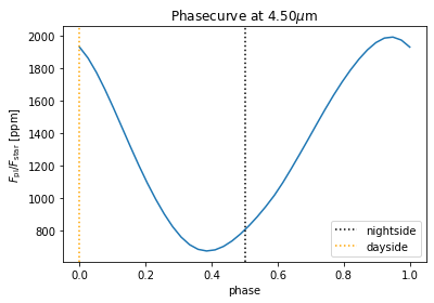
Lets create some phase curves!
[16]:
# 4.5 mu m plot
l = 4.5
idx = np.argmin(abs(wlen < l))

plt.plot(phases, flux[:,idx]*1e6)
plt.axvline(0.5, label='nightside', ls=':', color='black')
plt.axvline(0.0, label='dayside', ls=':', color='orange')
plt.xlabel('phase')
plt.ylabel(r'$F_\mathrm{pl}/F_\mathrm{star}$ [ppm]')
plt.title(r'Phasecurve at {:.2f}$\mu$m'.format(wlen[idx]))
plt.legend()
plt.show()

# 3.6 mu m plot
l = 3.6
idx = np.argmin(abs(wlen < l))
plt.plot(phases, flux[:,idx]*1e6)
plt.axvline(0.5, label='nightside', ls=':', color='black')
plt.axvline(0.0, label='dayside', ls=':', color='orange')
plt.xlabel('phase')
plt.ylabel(r'$F_\mathrm{pl}/F_\mathrm{star}$ [ppm]')
plt.title(r'Phasecurve at {:.2f}$\mu$m'.format(wlen[idx]))
plt.legend()
plt.show()